Diffusion Equation in Biology Explained: Interactive Graph & a 1950 Japanese Textbook

Why do molecules spread out, and how can an equation describe that movement inside a cell? To answer, we can open a Japanese mathematical biology textbook from 1950, follow its diffusion equations, and then experiment with an interactive graph. No calculus background is required to begin.

A 1950 time capsule: mathematics inside living cells

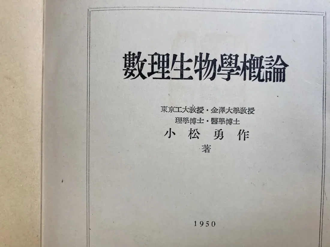
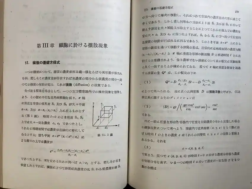
Sūri Seibutsugaku Gairon (數理生物學概論, “An Introduction to Mathematical Biology”) was written by Yūsaku Komatsu (小松勇作). Its title page is dated 1950; the photographed colophon records a third printing in March 1951. The book is more mathematical than its gentle title might suggest: Chapter III, “Diffusion Phenomena in Cells,” proceeds through concentration fields, flux, conservation laws, boundary conditions, and models of cellular growth.

It is a reminder that quantitative biology did not begin with modern computers. Researchers were already using differential equations to describe living systems long before today’s interactive software and molecular simulations.

1. Diffusion starts with a simple observation

Imagine putting a drop of dye into water. At first, the color is concentrated in one place. Over time, random molecular motion spreads it outward. That spreading process is diffusion.

If one region has more molecules per unit volume than the region next to it, there is often a net movement from the higher concentration toward the lower concentration. Individual molecules still move in both directions; the net flow is what matters.

2. Fick’s law: one minus sign with a big meaning

In one spatial dimension, Fick’s first law is written:

J = −D × (dc/dx)

Read it slowly: J is the net amount crossing a unit area each second; D tells us how readily the substance spreads; and dc/dx says how quickly concentration changes from one position to another. The minus sign means that the net flux points toward lower concentration.

Here is a tiny example with ordinary arithmetic. Suppose concentration falls from 10 to 6 units over a distance of 2 units. The change is 6 − 10 = −4. Divide by the distance: −4 ÷ 2 = −2. If D = 3, then flux is −3 × (−2) = +6, toward the positive x-direction.

Fick published an early systematic diffusion treatment in 1855, long before the 1950 textbook. See his original article, Ueber Diffusion, doi:10.1002/andp.18551700105.

3. The diffusion equation: how a curve changes over time

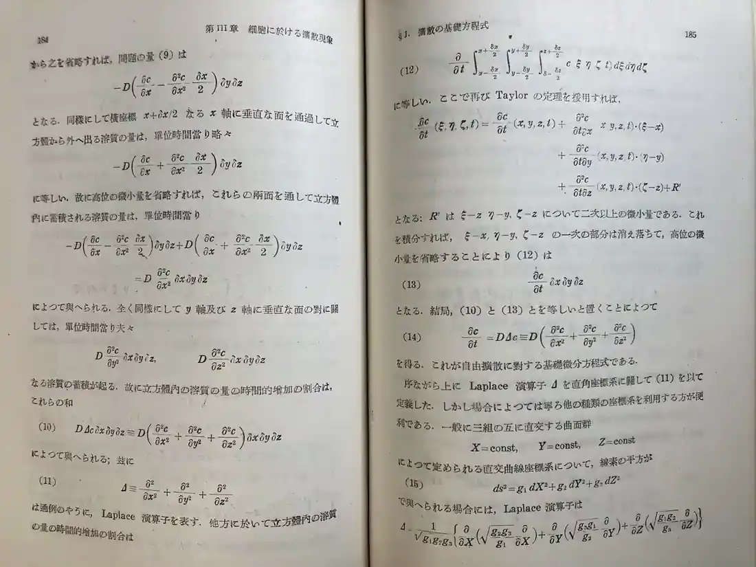
When we combine Fick’s law with conservation of material, we obtain the one-dimensional diffusion equation for constant D:

∂c/∂t = D × ∂²c/∂x²

The left side asks, “How fast is concentration changing here?” The right side uses the curvature of the concentration profile to answer. A sharp peak tends to flatten, and a low point between two higher regions tends to fill in.

The next graph uses a Gaussian starting profile spreading on an ideal infinite line. Its total amount is fixed and there is no chemical reaction, active transport, or membrane barrier. Change the sliders to see a physical equation become a moving picture.

4. What does the scary symbol ∂²/∂x² actually do?

It is simply a way to ask whether a concentration profile bends upward or downward. We can approximate that curvature using three neighboring numbers, without learning calculus first.

Suppose concentrations at left, center, and right are 4, 10, and 4, with equal spacing of 1 unit. The curvature estimate is:

(left − 2 × center + right) ÷ (spacing × spacing)

Put the numbers in: (4 − 2 × 10 + 4) ÷ (1 × 1) = −12. A negative number means the center is a peak that tends to fall as diffusion proceeds.

Replace the center with 2, keeping the neighbors at 4, and the result is (4 − 2 × 2 + 4) = +4: a dip that tends to rise. The interactive calculator below performs every arithmetic step for you.

5. Sigma (Σ) and the Laplacian (∇²): addition first, symbols second

A capital sigma, Σ, is shorthand for adding several things. For example:

Σ from i = 1 to 4 of i = 1 + 2 + 3 + 4 = 10.

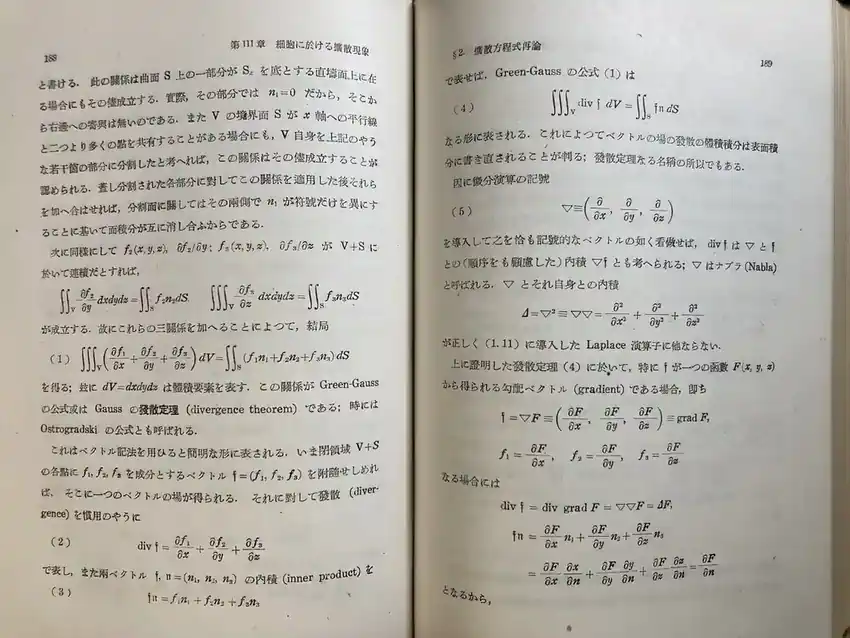
For a concentration that changes in three dimensions, the Laplacian adds the curvature along the x, y, and z directions:

∇²c = (∂²c/∂x²) + (∂²c/∂y²) + (∂²c/∂z²).

This is not mysterious multiplication. In Cartesian coordinates, it is three curvature measurements added together. In a computer, these derivatives can be approximated with neighboring values. Different geometries and boundary conditions require different numerical care.

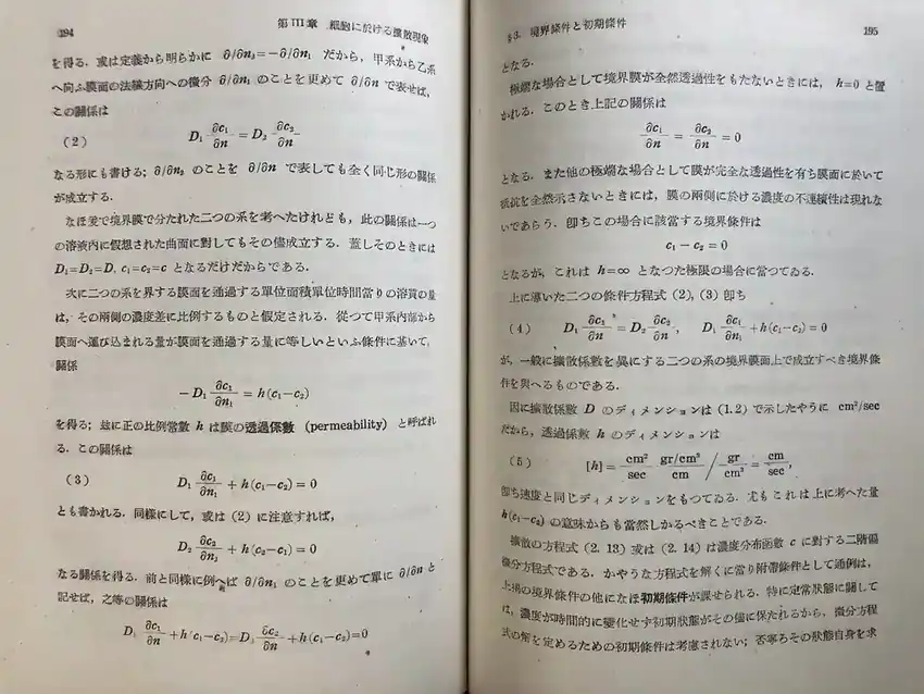
6. Boundaries matter: a cell is not an infinite glass of water

Real cells have membranes, organelles, binding sites, reactions, and moving boundaries. A no-flux boundary can be useful as a teaching assumption when material cannot cross the boundary. A permeable membrane requires a different condition. Because of these differences, the same diffusion coefficient may produce very different behavior in different systems.

The 1950 text devotes serious attention to boundary conditions and changing cell size. That is precisely where its old mathematics starts looking like today’s transport modeling: writing an equation is only the first step; the physical assumptions determine what the equation means.

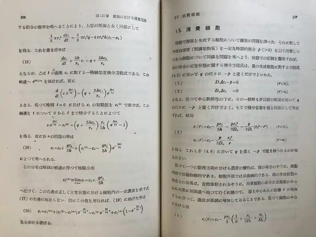
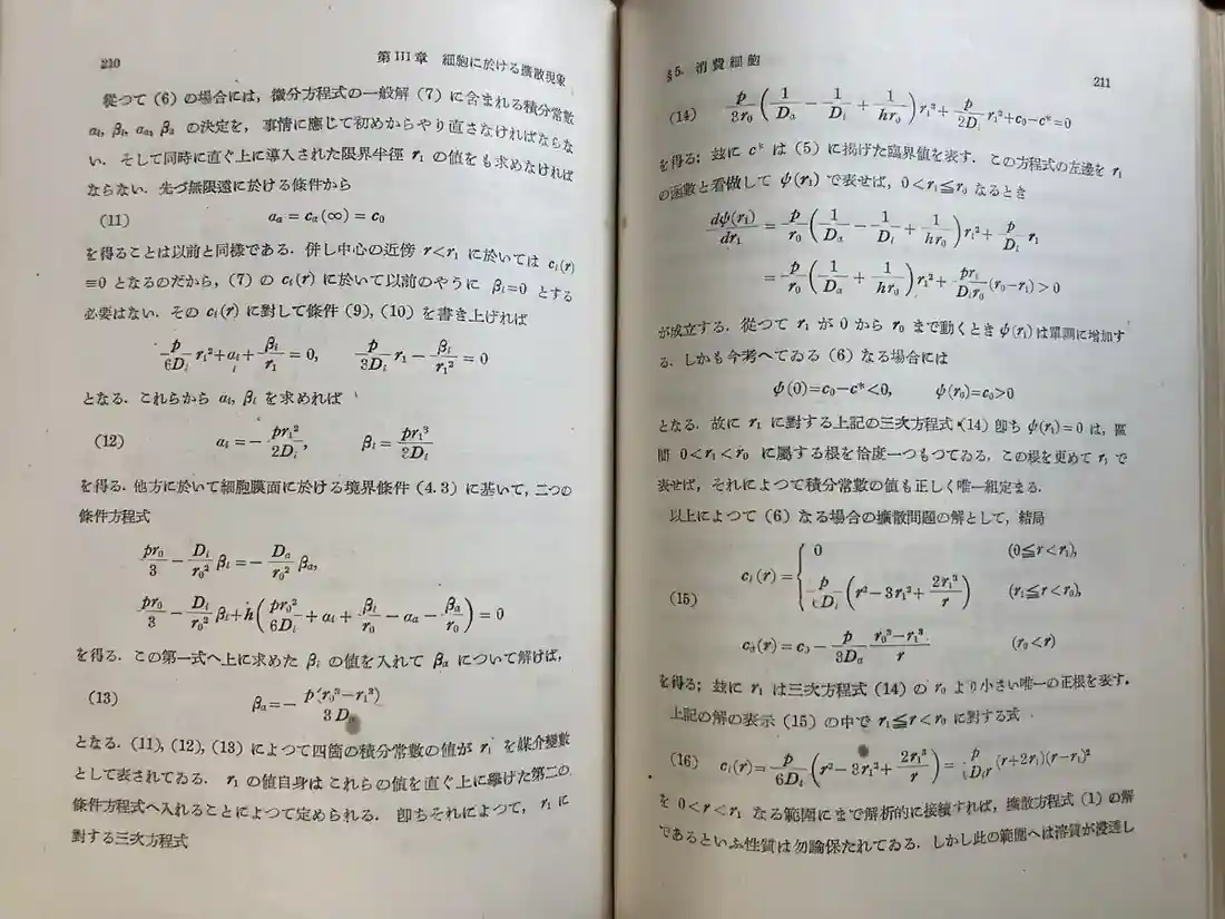
7. From 1950 to today: diffusion, patterns, and quantum chemistry

Two years after the book’s title-page date, Alan Turing published The Chemical Basis of Morphogenesis (1952). The argument was not simply that chemicals diffuse: under particular reaction and diffusion conditions, initially uniform systems can become unstable and develop spatial patterns. That is a reaction–diffusion problem, not the same as the spreading-only graph above. doi:10.1098/rstb.1952.0012.

Today, physical models span multiple scales. Diffusion equations describe changes in concentration in space and time. Quantum chemistry tools such as Psi4 instead calculate electronic structure for molecules, providing quantities such as energies and charge-related properties under specified theoretical approximations. They do not directly solve the same biological diffusion problem. Their connection is methodological: both force researchers to turn an assumption about nature into a mathematical model whose limitations can be tested.

A separate BCC Magazine article will cover a practical 2026 chemoinformatics and quantum-chemistry workflow using Psi4, molecular descriptors, and reproducible Python environments.

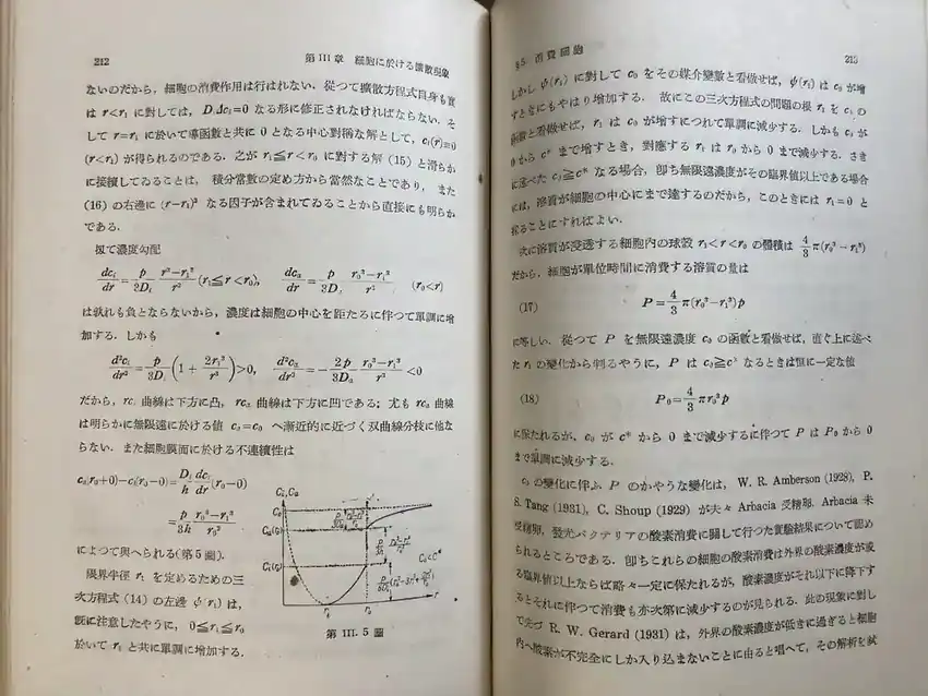
What should you remember?

Three ideas are enough to start. First, net diffusion follows concentration gradients. Second, the rate at which a profile changes depends on its curvature and on D. Third, boundaries and reactions change the answer. Once you understand these ideas, a page of symbols becomes less like an obstacle and more like a compact description of a physical story.

The old textbook deserves more than a glance for its age. It shows quantitative thinking applied seriously to cells at a time when every curve and derivation had to be worked through without the convenience of a browser slider.

Sources

1. Komatsu Y. Sūri Seibutsugaku Gairon (數理生物學概論). Title page dated 1950; third printing dated March 5, 1951. Historical source photographed here.
2. Fick A. Ueber Diffusion. Annalen der Physik. 1855;170(1):59–86. doi:10.1002/andp.18551700105.
3. Turing AM. The Chemical Basis of Morphogenesis. Philosophical Transactions of the Royal Society of London B. 1952;237(641):37–72. doi:10.1098/rstb.1952.0012.